Step-by-Step Guide: How to Lock Cells in MS Excel

Understanding Cell Locking in Excel

Locking cells in Microsoft Excel is a useful feature that allows you to protect important data from being altered. By default, all cells in an Excel worksheet are locked, but this setting only takes effect when the worksheet is protected. In this guide, we will walk you through the step-by-step process to lock cells effectively.

Step 1: Select the Cells You Want to Lock

Begin by opening your Excel file. Click and drag to highlight the cells that you wish to lock. If you want to lock the entire worksheet, simply press Ctrl + A to select all cells.

Step 2: Adjust Cell Lock Settings

With your desired cells selected, right-click to open the context menu and choose Format Cells. In the Format Cells window, navigate to the Protection tab. Here, you will see an option labeled Locked. Make sure this box is checked, then click OK.

Step 3: Protect the Worksheet

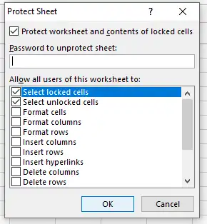
Now that your cells are marked for locking, it’s time to protect the worksheet. Go to the Review tab in the Excel ribbon and click on Protect Sheet. You can enter a password (optional) which will add an extra layer of security. Click OK, and your selected cells are now locked!

Following these steps will ensure that your important data remains intact and secure, providing peace of mind while working in Microsoft Excel.